
Anomaly Detection With Machine Learning, A Practical Playbook For Reducing Alert Noise
Anomaly detection with machine learning works in production only when you treat it as an end-to-end decision system: choose the right learning setup, engineer noise-resistant features, and calibrate thresholds to match your false-positive budget.
- Choose supervised, semi-supervised, or unsupervised based on label quality, drift rate, latency, and acceptable false-positive burn.
- Reduce noise before modeling with segmentation, explicit missingness handling, seasonal baselines, and residual-based features.
- Convert scores to actionable alerts using per-segment thresholds, adaptive calibration, and incident-window evaluation (not point metrics).
Choose the right anomaly detection setup, supervised vs semi-supervised vs unsupervised
Anomaly detection with machine learning becomes noisy when the learning setup does not match your labeling reality, novelty rate, and on-call tolerance for false alarms.
Decision table for picking a setup
Use the table below as an if-then selector. The “best” setup is the one that minimizes expected interruption cost while still catching incidents inside your detection latency target.
| Constraint | Supervised | Semi-supervised (learn normal) | Unsupervised |
|---|---|---|---|
| Label availability | Reliable incident labels, stable definitions | Mostly-normal history, sparse incidents | No labels or labels too noisy |
| Failure novelty | Low to moderate recurring patterns | Moderate to high, new incidents likely | High unknown unknowns |
| Drift / seasonality | Retrain after product changes | Can update “normal” with safeguards | Often brittle without segmentation |
| Latency requirement | Low (fast inference) | Low to medium (window features) | Medium (often needs clustering/windows) |
| False-positive budget | Lowest if labels reflect real cost | Good if thresholding is disciplined | Highest risk without guardrails |
| Best first use | Top 3 to 10 recurring incident classes | Service metrics, key user flows | Offline discovery and triage support |
Heuristics that prevent noisy deployments
- Do not do supervised unless your labels map to “actionable.” If your historical “incidents” include expected business failures (declines, validation errors), you will train the model to alert on expected outcomes.
- Prefer semi-supervised for monitoring-style telemetry. When incidents are rare, learning a baseline of “normal” and flagging deviations usually beats trying to learn a brittle incident classifier.
- Use unsupervised to find segments, not to page people. In practice, unsupervised methods are great at surfacing “weird” cohorts (a country, endpoint, or app version) that you then model or threshold more carefully.
A simple selection checklist
- Can you write a one-sentence label definition that an on-call engineer would accept at 3 a.m.?
- How often do new product releases change the data distribution for this metric or flow?
- What is your acceptable false-positive burn: how many pages per day/week before engineers start ignoring the channel?
- Do you need explanation (why flagged) for triage, or is a single score enough?
Build a real-world feature pipeline that reduces noise before modeling
Feature engineering for anomaly detection with machine learning should remove predictable variation first, because models trained on raw seasonality and missingness will “detect” your calendar and your instrumentation bugs.
Start with segmentation, not a single global model
Segmentation is the cheapest noise reducer. Common segments in monitoring data include service, endpoint, region, customer tier, app version, and deployment ring. A practical rule: if two segments have different baselines or different acceptable error rates, they should not share one threshold.
- Good segments: /api/checkout vs /api/search, iOS vs Android, EU vs US, free vs paid tier.
- Bad segments: user_id (too sparse), session_id (too volatile), anything that explodes cardinality without stable baselines.
Handle missingness explicitly
Missing data is often more informative than a value. Add explicit “is_missing” flags, and distinguish “no traffic” from “no telemetry.” For counters, use a fill strategy that matches semantics: forward-fill gauges, but do not forward-fill rates if a pipeline outage is plausible.
Remove seasonality with residual features
Residual-based features are a reliable default: model or estimate the expected value, then run anomaly detection on the residual (actual minus expected) rather than on the raw metric.
- Baseline options: hourly/weekly seasonal medians, STL decomposition, or a simple forecasting model where appropriate.
- Residual features: residual, absolute residual, residual z-score using a rolling robust scale (median absolute deviation).
When we audited a noisy alert stream for a consumer app, the biggest win was replacing raw error counts with “errors minus expected errors for this hour-of-week,” which removed predictable peaks and reduced nuisance alerts without changing the model class.
Use rolling windows that match incident shape
Choose windows based on how incidents manifest. Spikes need short windows (1 to 5 minutes), slow regressions need longer (30 to 120 minutes), and many systems benefit from multi-scale features.
- Window features: rolling mean, rolling max, rolling percentile, slope (linear trend), and change-point proxies (difference of rolling means).
- Context features: deploy marker, traffic volume, queue depth, and saturation metrics, because “same error rate” means different impact at different traffic.
Concrete pipeline checklist (minimum viable)
- Define the event or metric and the unit of analysis (endpoint-level rate, checkout funnel step failure rate, latency p95).
- Choose 2 to 4 stable segments.
- Compute traffic-aware rates (errors/requests) and carry raw denominators.
- Add missingness flags and a telemetry-health signal.
- Create residual features vs hour-of-week baseline.
- Generate 2 to 3 rolling windows aligned with your paging latency.
Model selection for anomaly detection with machine learning, reliable defaults and failure modes
Model choice for anomaly detection with machine learning should be driven by data shape and explainability needs, because the best-performing offline model can still fail operationally if engineers cannot validate why it fired.
Reliable defaults by data type
- Single metric with seasonality: residual thresholding or forecasting + residual scoring (simple baselines often outperform complex models for alerting).
- Many correlated metrics: PCA-style reconstruction error, autoencoder reconstruction error, or robust covariance approaches, with careful scaling.
- Event-level records with mixed types: tree-based models for supervised or semi-supervised scoring, or density-based methods offline for exploration.
What tends to break in production
- Isolation Forest: sensitive to contamination assumptions; can drift as traffic mix changes; scores are not calibrated probabilities.
- One-class SVM: expensive at scale and sensitive to feature scaling; works best on smaller, well-behaved feature sets.
- Autoencoders: can learn to reconstruct anomalies if training data is contaminated or if retraining is too frequent without holdouts; harder to explain without auxiliary signals.
- Clustering-based outliers: often unstable when cardinality changes (new endpoints, new regions), leading to repeated “new cluster” alerts.
Interpretability hooks that lower alert noise
Regardless of algorithm, bake in “why” signals that help a human validate quickly:
- Top contributing features (for linear models, trees, or SHAP-like summaries when feasible).
- Residual plots vs expected baseline and recent history window.
- Segment diff (which region/version is driving the deviation).
- Denominator checks (requests, users) to prevent “rate anomalies” from tiny traffic.
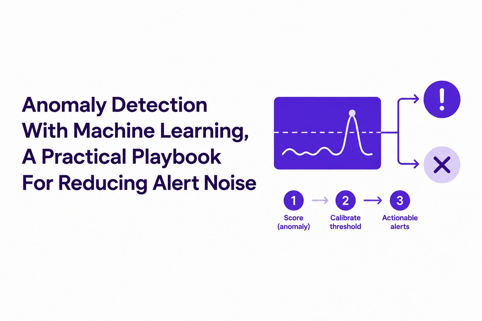
Thresholding and alert calibration playbook, turn scores into actionable alerts
Thresholding is where anomaly detection with machine learning succeeds or fails, because an excellent scorer with a naive cutoff still becomes a false-positive generator.
Start with a cost-based threshold, not a percentile
If you can estimate costs, pick thresholds using expected cost:
- Cost of false positive: engineer interruption, context switching, follow-up work.
- Cost of false negative: user impact, revenue risk, SLA breach, reputational risk.
Even a rough ratio helps. For example, if a missed checkout outage is far more expensive than a nuisance page, you tolerate a higher alert rate for that segment than for a low-impact endpoint.
Practical threshold methods and when to use them
- Static percentile on residuals: good for stable metrics with clear baselines; brittle under drift.
- Contamination/nu-style parameters: useful when you believe a fixed fraction of history is anomalous; dangerous if incident frequency changes.
- Adaptive thresholds: compute dynamic cutoffs per hour-of-week or via rolling quantiles; best for strong seasonality.
- Two-stage gating: first gate on “impact” (denominator, affected users), then gate on anomaly score; this reduces noisy low-traffic alerts.
Per-segment tuning without exploding complexity
Use a small number of threshold tiers rather than fully bespoke tuning:
- Tier A (high impact): checkout, auth, core APIs, high-revenue flows.
- Tier B (medium impact): search, recommendations, secondary flows.
- Tier C (low impact): optional assets, best-effort integrations.
Each tier gets a different false-positive target and severity mapping. This keeps anomaly detection with machine learning aligned with business impact instead of treating all deviations equally.
Alert design that prevents duplicate storms
- Group by fingerprint: one issue per root cause signature, with an occurrence counter, rather than hundreds of pages.
- Use hold-down timers: once an alert fires, suppress repeats for a fixed window unless severity increases.
- Require persistence: alert only if score exceeds threshold for N out of M points (for noisy metrics).
We initially assumed “lower threshold catches incidents earlier,” but our team found persistence rules (N out of M) often cut pages dramatically while keeping time-to-detect acceptable for real incidents.
Evaluate what matters in imbalanced incidents, PR-AUC, incident windows, and cost
Evaluation for anomaly detection with machine learning should be incident-based, because pointwise accuracy hides the operational reality of paging on windows and responding to grouped issues.
Use incident windows, not single timestamps
Define incidents as windows with a start and end (even if rough), and score detection as “did we alert within the window with acceptable delay.” A simple scheme:
- True positive: at least one alert within the incident window.
- Time-to-detect: first alert time minus incident start time.
- False positive: alert outside any incident window.
- Alert volume: total alerts and unique grouped issues.
Prefer PR curves to ROC in rare-incident settings
Precision-Recall curves are usually more informative than ROC when incidents are rare. Track precision at your target recall or recall at your maximum acceptable page rate.
Track a “false-positive burn rate”
Operationalize noise as a weekly budget: how many false alerts per service per week can your team handle before trust collapses. Then measure:
- FP/week by segment and severity
- Pages per on-call shift attributed to the detector
- Percent of alerts with a confirmed root cause (even “expected outcome” counts as root-cause, but should become a rule)
Offline-to-online evaluation bridge
- Run detectors in shadow mode for 1 to 2 weeks.
- Collect analyst labels on a small sample of alerts (actionable, expected, duplicate, low confidence).
- Recalibrate thresholds and add segmentation or impact gating before paging.
A minimal project template to ship anomaly detection into production
A production-ready anomaly detection with machine learning project needs a small, disciplined template so you can iterate on thresholds, drift, and routing without rebuilding everything.
Repo blueprint (minimal but complete)
- /data: feature definitions, segment configs, baseline computation code
- /models: training scripts, saved artifacts, scoring interface
- /calibration: threshold configs per tier/segment, persistence rules
- /evaluation: incident-window metrics, PR curves, time-to-detect reports
- /ops: deployment, schedules, drift checks, runbooks
Baseline-first checklist (what to ship before any fancy model)
- Seasonal baseline + residuals
- Impact gating (minimum traffic/affected users)
- Persistence rule (N out of M)
- Grouping and suppression to avoid duplicate storms
- Shadow mode report that shows top segments by alert volume
Drift and instrumentation monitoring
- Data drift: track changes in feature distributions per segment.
- Concept drift: track precision proxy, such as percent of alerts marked “expected outcome.”
- Telemetry health: missingness rate and pipeline lag, to avoid “detectors detecting the collector.”
Safe rollout plan
- Phase 1 (shadow): record alerts, no paging.
- Phase 2 (notify low severity): route to a quiet channel or daily digest.
- Phase 3 (page for Tier A only): limited segments, strict suppression, clear runbook.
- Phase 4 (expand): add segments and tighten thresholds based on measured false-positive burn.
| Step | Common failure | Fix that reduces noise |
|---|---|---|
| Setup choice | Unsupervised pages on “weird” but harmless patterns | Use unsupervised offline, deploy semi-supervised for paging |
| Features | Seasonality triggers daily false alarms | Residuals vs hour-of-week baseline |
| Thresholds | One global cutoff | Tiered per-segment thresholds + impact gating |
| Alert routing | Duplicate storms | Fingerprint grouping + hold-down timers |
| Evaluation | ROC looks good, on-call hates it | Incident-window precision, time-to-detect, FP/week |
FAQ
If you apply this playbook and want anomaly signals to translate into clean, actionable engineering issues instead of noisy alerts, Flash Log adds a decision layer that captures bugs automatically (even when users do not report them), groups duplicates, and classifies expected failures vs real production issues before they reach Jira, Linear, Slack, or reports.
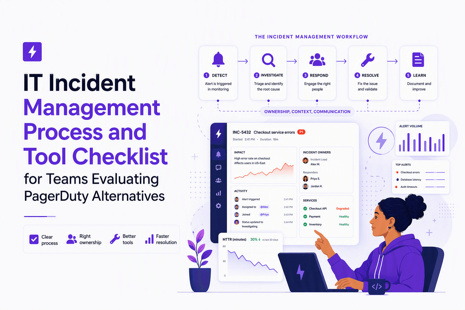
IT Incident Management Process and Tool Checklist for Teams Evaluating PagerDuty Alternatives
Build an it incident management process that maps each stage to tool requirements, major-incident roles, and integrations for PagerDuty-alternative evaluations.

Notification Fatigue Explained and a Simple Reset Plan You Can Finish This Week
Learn what notification fatigue is, how to diagnose it, and a practical reset plan for phone, email, chat, and social without going off-grid.

Alert Fatigue Fix, A 30 60 90 Day Playbook to Cut Noise and Improve On-Call
A practical 30/60/90-day playbook to reduce alert fatigue with KPIs, paging policy, and AI noise reduction you can prove in production.