
Anomaly Detection That Doesn’t Create Noise, A Practical Framework for Choosing Models and Thresholds
Anomaly detection works in production only when you define what “actionable” means, choose detectors that match your data, and set thresholds that control noise as aggressively as you control misses. The biggest failure mode I see is treating detection as a modeling problem instead of an operational system: the result is a flood of tickets, constant threshold tweaks, and teams that stop trusting alerts.
- Write an “actionable anomaly” definition first, then map it to point, contextual, or collective anomalies so you do not alert on statistical oddities with no owner.
- Pick models by data type and failure mode (time series vs tabular vs logs), and treat scoring and thresholding as separate decisions you can iterate independently.
- When you lack labels, evaluate with ranked review, backtesting on known incidents, weak labels, and cost-weighted metrics so you optimize for interruptions avoided, not just ROC curves.
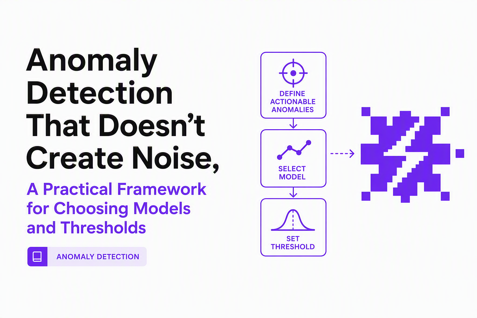
Start With the Right Problem Statement or Your Anomaly Detection Will Generate Noise
Anomaly detection generates noise when the system optimizes for “unusual” instead of “actionable,” so the first deliverable should be a crisp anomaly contract that links signals to decisions. In practice, that contract is one page: what you alert on, who owns it, how fast it must be acted on, and what evidence the alert must include to be triageable.
Use a three-way definition to prevent category mistakes
Teams often mix three related ideas, then wonder why the alert stream feels random:
- Outlier: a rare point in a dataset (often a data quality issue). Example: a negative latency, a duplicated ID, a malformed JSON payload.
- Anomaly: a deviation that suggests a system change worth investigating. Example: 500 rate rising above baseline for a specific route.
- Novelty: a new pattern not seen in training, often expected in evolving products. Example: a new user flow after a UI release; a new country rollout changes traffic mix.
The operational trap is treating novelty as anomaly, especially in fast-shipping teams. A good contract explicitly says whether you alert on novelty at all (often you should not), and if you do, which launches or segments warrant it.
Define “actionable anomaly” with four fields
To make “actionable” measurable, define it with fields you can check at review time:
- Impact: what user or business outcome is at risk (checkout completion, login success, API latency budget).
- Owner: which team is responsible (payments, platform, search). If no owner exists, do not alert by default.
- Time sensitivity: how quickly action matters (minutes for outages, days for slow data drift).
- Evidence package: what context must be attached (route, error class, sample requests, correlation IDs, release version).
In our experience, writing the evidence package up front cuts noise because it forces you to confront which anomalies are actually diagnosable. If you cannot attach enough context to act, route it to a daily review queue instead of paging on it.
Map the contract to point, contextual, or collective anomalies
Choosing the wrong anomaly shape is a common reason thresholds feel impossible to tune:
- Point anomalies: a single observation is abnormal (fraud score spike, a single sensor reading). Best when single events matter.
- Contextual anomalies: abnormal relative to context (time of day, region, device type). Best for seasonality and segment shifts.
- Collective anomalies: a pattern over a window is abnormal even if each point is not (a gradual latency climb, a burst of timeouts). Best for incidents.
If you are paging engineers, you are usually hunting collective anomalies (bursts, shifts, sustained elevations), not isolated odd points. That single choice will drive your windowing, features, and evaluation approach.
Model Selection Cheat Sheet by Data Type and Anomaly Type
Model selection for anomaly detection should start from the data you actually have at alert time, not the algorithm you prefer. The practical goal is a stable anomaly score that correlates with “worth waking someone up,” even if the model is simple.
Decision flow for picking 2 to 3 candidate detectors
- Identify data type: tabular metrics, time series, logs or text, images.
- Identify anomaly shape: point, contextual, collective (from your contract).
- Decide on latency: batch (hourly/daily) vs streaming (minutes/seconds).
- Decide on explainability needs: do responders need feature attributions, nearest neighbors, or example traces?
Cheat sheet by data type
- Tabular (events, user-level aggregates)
- Isolation Forest: strong default for mixed numerical features; scalable; outputs a continuous score that thresholds well.
- Local Outlier Factor (LOF): good for “locally rare” patterns; more sensitive to density changes; harder to use for streaming because scoring depends on neighborhood.
- One-Class SVM: can work on smaller, well-scaled datasets; can be brittle at scale and sensitive to kernel and nu choices.
- Time series (rates, latency percentiles, error counts)
- Seasonal baseline + residual threshold: often beats complex models for alerting. Use day-of-week and hour-of-day baselines, then alert on residuals.
- Change-point detection: best when you care about shifts (release regressions). Consider algorithms like PELT for batch detection, or CUSUM-style methods for streaming.
- Forecasting residuals: ARIMA/ETS or modern methods when seasonality is strong and you can maintain model fits.
- Logs and text (error messages, stack traces)
- Fingerprinting + frequency anomalies: group similar logs, then detect spikes in grouped counts.
- Embedding + density or clustering: embed messages, cluster, and flag new clusters or drift; operationally heavier, but useful when message variety is high.
- Images (visual QA, manufacturing)
- Autoencoder reconstruction error: common when you have many “normal” images.
- Pretrained feature embeddings + kNN: often practical and explainable by nearest neighbors; tune threshold on distances.
Selection criteria that matter more than leaderboard performance
- Score stability: the same situation should produce similar scores across days, otherwise thresholding becomes whack-a-mole.
- Segmentability: can you compute scores per route, per tenant, per region without retraining everything?
- Debuggability: can responders answer “why did this fire” with features, examples, or comparisons?
- Operational cost: retraining frequency, feature pipelines, and the ability to backfill and reproduce results.
When we tested Isolation Forest against LOF on product analytics aggregates, the deciding factor was not raw hit rate but threshold stability after new feature launches. LOF produced more “locally weird” findings that were interesting but rarely actionable; Isolation Forest produced fewer, higher-signal alerts that matched owners and runbooks.
Thresholding and Anomaly Scoring Without Alert Fatigue
Thresholding is where anomaly detection either becomes a trusted signal or turns into alert fatigue, so treat thresholds as a policy decision tied to interruption budgets. A good threshold is not “mathematically correct,” it is the one that keeps pages rare, reviews manageable, and incidents caught early enough to matter.
Separate scoring from alerting with a two-tier policy
Use the model score to rank anomalies, then apply two different thresholds:
- Page threshold: high precision, low volume. Fires only when impact and confidence are both high.
- Review threshold: lower precision allowed. Populates a daily or weekly queue for humans to sample.
This single design choice dramatically reduces noise because you stop forcing one threshold to satisfy two different workflows.
Three practical ways to set thresholds without labels
- Quantile thresholds: pick a target rate, like “top 0.1% most anomalous per day per service,” then adjust. This is easiest when volume is stable.
- Contamination parameter: for models like Isolation Forest, set expected anomaly fraction (for example 0.01) to shape the score distribution. Treat it as a knob, not a truth.
- Seasonal baselines: for time series, compute residuals vs expected value for the same hour-of-week, then threshold residual magnitude. This prevents “Monday traffic is higher” alerts.
Route by severity to avoid everyone getting pinged for everything
Thresholds should be conditional on impact and ownership, not global. A pragmatic scheme:
- Severity 1: affects core journey completion (payments, auth) and sustained over a window. Page.
- Severity 2: user-visible degradation but with workarounds. Slack alert or ticket.
- Severity 3: suspicious but low-confidence or low-impact. Review queue only.
Connect this to an alert management policy so routing and escalation are consistent with on-call expectations.
Noise controls that beat more modeling
- Deduplication windows: group repeated firings into one incident thread (for example, one alert per fingerprint per 30 minutes) so storms do not create ticket floods.
- Suppression rules: mute known expected failures (rate limits, validation errors) unless their rate changes drastically.
- Cooldowns and hysteresis: require sustained recovery before resolving, and sustained degradation before firing, to avoid flapping.
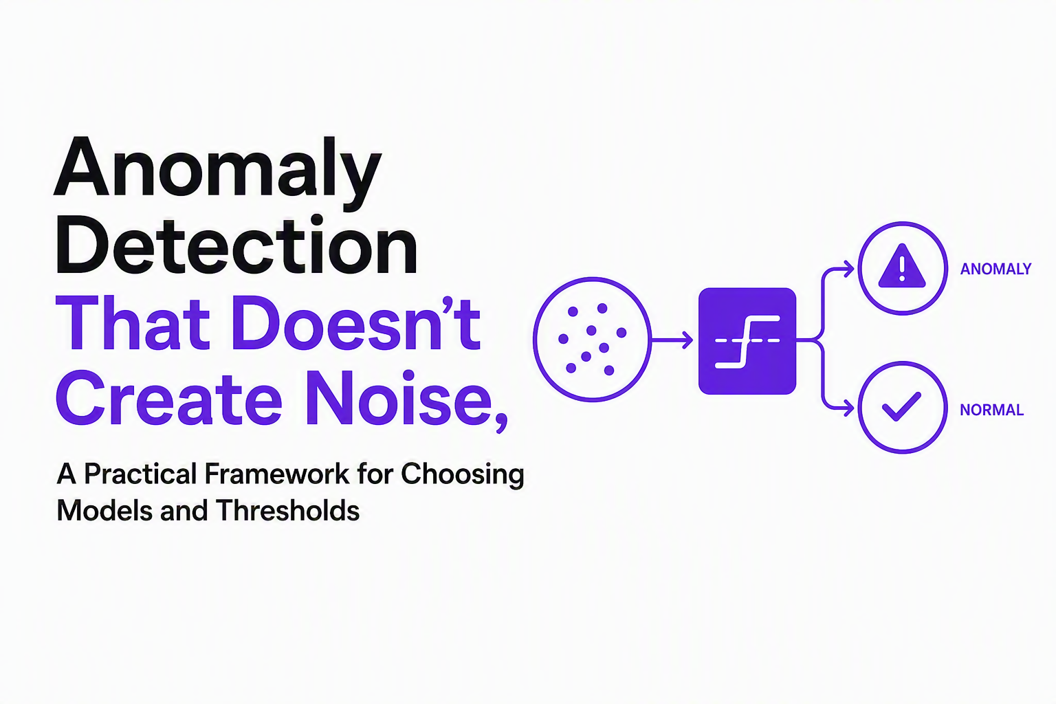
Evaluate Unsupervised Anomaly Detection When You Don’t Have Labels
Evaluation without labels is doable if you treat anomaly detection as a ranking problem plus a cost problem, not a binary classifier. The goal is to prove that the top of the ranked list contains a higher concentration of actionable issues than random sampling, and that alert volume stays within your interruption budget.
Use ranked review as your primary offline metric
Create a weekly evaluation loop:
- Score all candidates and rank descending by anomaly score.
- Sample the top N (for example top 50) and a random baseline sample (for example 50 random points).
- Have reviewers label each as “actionable,” “expected,” or “unclear,” plus owner and severity.
- Track actionable rate in top N vs random. If top N is not materially better, your detector is not ranking well.
This produces weak labels over time and focuses effort where it matters: the alerts people actually see.
Backtest against known incident windows and releases
Even if you lack per-event labels, you usually know incident timestamps, deploy timestamps, and major config changes. Backtest by asking:
- Did scores elevate before or during known incident windows?
- Did the system spike on deploys that were harmless (false alarms), or only on deploys correlated with regressions?
A lightweight way is to compute “average anomaly score” in a fixed window after deploy and compare across deploys, then investigate outliers. You can do this for each service or endpoint to find where the detector is trustworthy.
Measure cost-weighted performance, not just hit rate
Operationally, a false positive costs interruptions, while a miss costs downtime or user harm. A simple, defensible rubric:
- FP cost: time to triage (for example 5 to 15 minutes) times number of responders interrupted.
- FN cost: estimated time-to-detect delay times incident impact tier.
Use the rubric to compare threshold settings: if lowering a threshold adds 30 extra pings per week but only catches one low-impact issue earlier, you should not do it.
Calibrate reviewers and definitions to avoid label drift
Review labels drift when “actionable” quietly changes. Keep a short labeling guide with examples, and run occasional double-review on a small sample to ensure consistency. In our experience, the biggest evaluation failures came from inconsistent severity definitions across teams, not from the model itself.
A Reproducible Python Walkthrough From Data to Deployment-Ready Outputs
A deployment-ready anomaly detection workflow produces a score, a thresholded decision, and enough context to reproduce the finding later. The example below uses standard scikit-learn style methods and keeps the focus on: feature prep, scoring, threshold selection, and packaging outputs for downstream alerting.
1) Prepare data and a sane baseline
Assume you have a pandas DataFrame of request aggregates per endpoint per 5-minute window:
# columns example
# ['ts', 'service', 'endpoint', 'req_count', 'err_5xx', 'p95_ms', 'region']

# typical features
df['err_rate'] = df['err_5xx'] / df['req_count'].clip(lower=1)
Before modeling, build a baseline residual for time-of-week if you have seasonality:
# pseudo-code: compute expected err_rate by (endpoint, day_of_week, hour)
Even a simple baseline often removes 80% of “expected variance” that would otherwise become noise, and it makes your ML detector’s job easier.
2) Fit three unsupervised detectors on tabular features
from sklearn.ensemble import IsolationForest
from sklearn.neighbors import LocalOutlierFactor
from sklearn.svm import OneClassSVM
from sklearn.preprocessing import StandardScaler
import numpy as np

features = ['err_rate', 'p95_ms', 'req_count']
X = df[features].values
X = StandardScaler().fit_transform(X)

iso = IsolationForest(n_estimators=200, contamination=0.01, random_state=42)
iso.fit(X)
iso_score = -iso.score_samples(X)  # higher = more anomalous

# LOF: fit_predict gives -1 for outliers; use negative_outlier_factor_ as score
lof = LocalOutlierFactor(n_neighbors=35, contamination=0.01)
lof_flag = lof.fit_predict(X)
lof_score = -lof.negative_outlier_factor_

oc = OneClassSVM(nu=0.01, kernel='rbf', gamma='scale')
oc.fit(X)
oc_score = -oc.score_samples(X)
Notes that matter in practice:
- Standardize features, otherwise p95_ms can dominate.
- Keep contamination/nu aligned across models so score tails are comparable.
- Do not compare raw scores across different model families without calibration; compare ranked lists.
3) Choose thresholds with quantiles and confirm with human review
# Example: review threshold at 99.5th percentile, page threshold at 99.9th
review_thr = np.quantile(iso_score, 0.995)
page_thr = np.quantile(iso_score, 0.999)

df['iso_review'] = iso_score >= review_thr
df['iso_page'] = iso_score >= page_thr
Then, validate the top ranked items by endpoint. If the top list is dominated by a single noisy endpoint, that is a segmentation problem, not a modeling problem. Split the detector per endpoint group or add endpoint as a grouping key and score within group.
4) Package output as a triageable alert payload
To make detections actionable, ship an object that includes context and a stable grouping key:
alert = {
  "ts": str(df.loc[i, 'ts']),
  "service": df.loc[i, 'service'],
  "endpoint": df.loc[i, 'endpoint'],
  "score": float(iso_score[i]),
  "decision": "page" if df.loc[i, 'iso_page'] else "review",
  "evidence": {
    "err_rate": float(df.loc[i, 'err_rate']),
    "p95_ms": float(df.loc[i, 'p95_ms']),
    "req_count": int(df.loc[i, 'req_count'])
  },
  "fingerprint": f"{df.loc[i,'service']}|{df.loc[i,'endpoint']}|err_rate"
}
That fingerprint becomes the key for dedupe and for tracking recurrence across time windows.
Production Blueprint for an Anomaly Detection System That Improves Over Time
A production anomaly detection system stays accurate by combining detection, noise control, and feedback into one loop you can run every week. The common anti-pattern is shipping a model and then only touching it when on-call complains, which guarantees thrash and mistrust.
Reference architecture for batch and streaming
- Ingest: metrics, traces, logs, and business events land in a warehouse or stream.
- Feature layer: computed aggregates, seasonal baselines, and segment keys (service, endpoint, tenant).
- Scoring service: runs batch (hourly) or streaming; produces anomaly scores plus evidence.
- Noise gate: dedupe, suppression rules, confidence thresholds, severity routing.
- Workflow outputs: tickets, Slack, paging, and a review queue for low-confidence signals.
- Feedback store: reviewer labels, incident links, and outcomes (fixed, ignored, expected).
Launch checklist that prevents most early failures
- Set an interruption budget: how many pages per week per team is acceptable.
- Define ownership mapping: every alert route must map to a team and a runbook.
- Implement grouping: one issue per fingerprint with occurrence counts, not one per event.
- Stand up a review queue: ensure low-confidence items still get sampled for learning.
- Schedule evaluation: weekly ranked review and monthly threshold calibration.
Handle drift with segmentation and recalibration, not constant retraining
Drift often shows up first as “everything looks anomalous” after a product change. The fastest fixes are usually:
- Segment more finely: new cohorts (region, plan, device) may need separate baselines.
- Recompute baselines: seasonal residual approaches need periodic baseline refresh.
- Recalibrate thresholds: quantile thresholds should be revisited if volume changes materially.
We initially assumed retraining weekly would solve drift, but operational data showed that segmentation and baseline refresh removed most false alarms with far less complexity. Retraining helped only after the data definition itself was stable.
Connect detection to fast debugging and resolution
Detection is only the start. A lot of time is burned after an anomaly is found: reproducing the bug, finding the relevant logs, and deciding whether it is expected behavior or a real defect. If you want anomaly detection to create business impact, invest in the handoff: grouped issues, attached context, and consistent alert triage routines, plus a standard way to mark expected outcomes and false positives so the system learns.
| System choice | What it optimizes | Typical failure mode | Noise-control fix |
|---|---|---|---|
| Global threshold for all services | Simplicity | One noisy service dominates alerts | Segment thresholds by service/endpoint |
| Point anomaly detector on incident data | Rare-event spotting | Misses sustained degradations | Windowed or change-point detection |
| High-sensitivity paging | Catch everything | Responders stop trusting pages | Two-tier thresholds: page vs review |
| ML-only pipeline | Automation | Unexplainable alerts, hard tuning | Rules for known expected failures + ML for the rest |
FAQ
If you want anomaly signals to translate into faster fixes, pair detection with automatic capture and classification of the underlying production bugs so engineers do not spend cycles reproducing what users never reported. Flash Log adds that operational layer by capturing bugs automatically even when users do not file reports and classifying them so the team can move from anomaly to actionable issue with less investigation time. Try Flash Log to operationalize the feedback loop after anomalies are found.

Stack Trace Explained, How To Read It And What To Collect When It’s Not Enough
Learn what a stack trace is, how to read it, and what context to collect when a stack trace isn’t enough to fix production bugs.
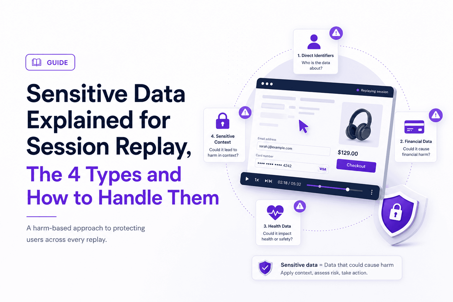
Sensitive Data Explained for Session Replay, The 4 Types and How to Handle Them
Learn what sensitive data means for session replay, a 4-type taxonomy, and a discover → classify → mask → retain workflow to reduce privacy risk.
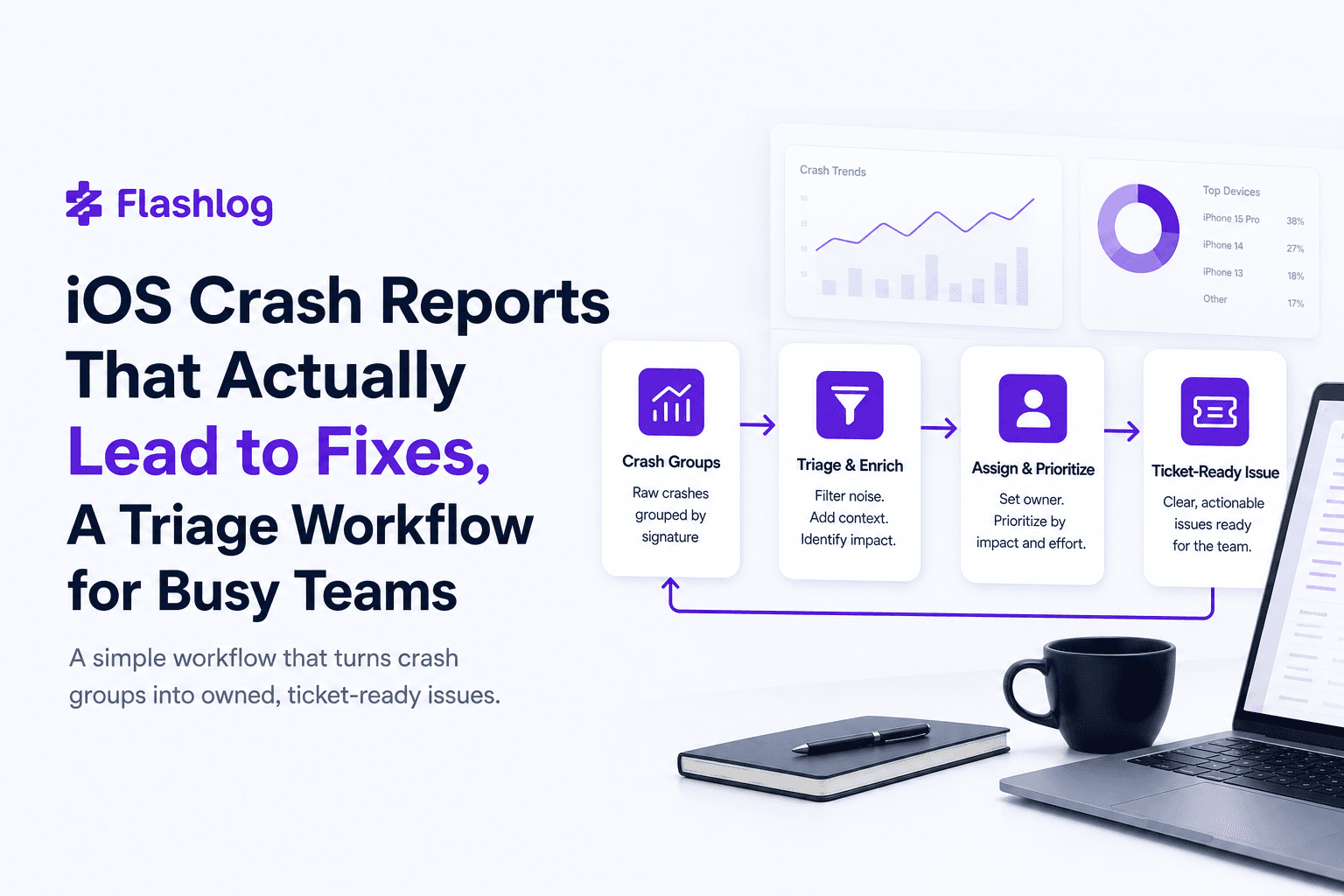
iOS Crash Reports That Actually Lead to Fixes, A Triage Workflow for Busy Teams
Turn ios crash reports into actionable tickets with a simple triage rubric and a minimum context bundle your iOS team can trust.