
Machine Learning Anomaly Detection That Reduces Alert Noise, Models, Thresholds, and Examples
Machine learning anomaly detection reduces alert noise when you first map anomaly type to data shape, then choose a model that matches your assumptions, and finally tune thresholds against precision and operational cost instead of gut feel.
- Start by classifying anomalies (point, contextual, collective) and aligning them to tabular, time-series, or logs/text so you do not pick a mismatched model.
- Model choice is mostly about assumptions you can defend in production: feature independence, seasonality, sparsity, and label availability.
- Thresholding and evaluation are where false positives are won or lost; use PR-focused metrics, top-k review, and cost-based gates.
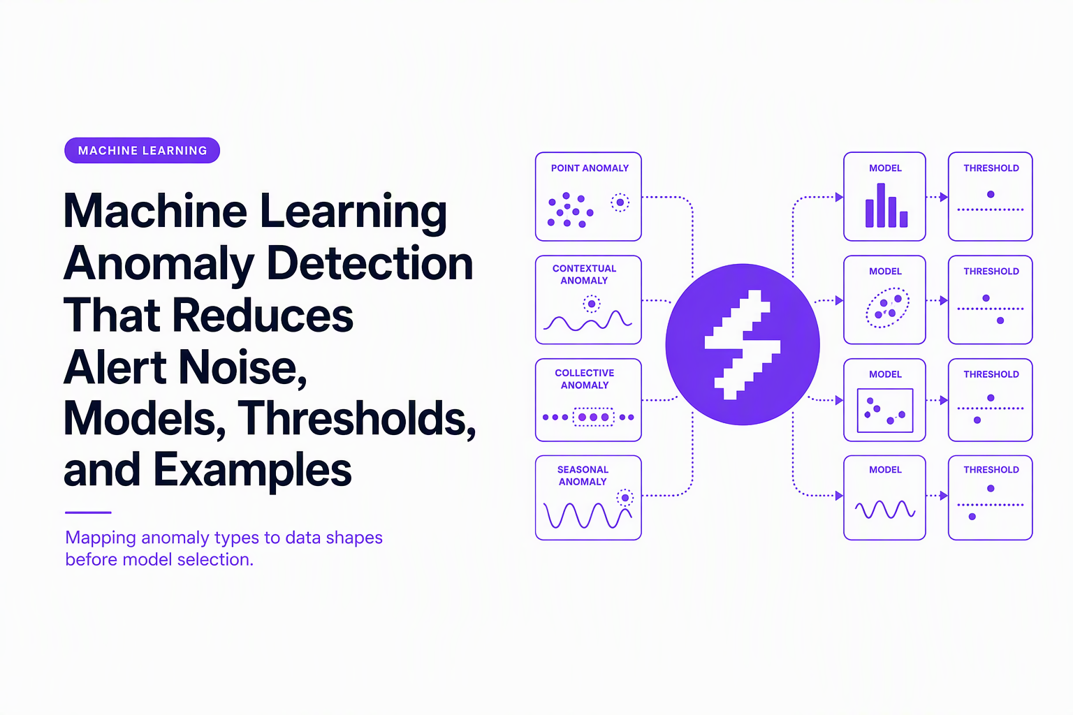
Map Your Anomaly Type and Data Shape Before Picking a Model
Model selection for machine learning anomaly detection becomes straightforward once you explicitly map (1) anomaly type and (2) data shape to the failure mode you care about in production.
Step 1: Classify the anomaly as point, contextual, or collective
- Point anomaly: a single record is weird by itself (ex: impossible combination of features, one request latency 100x baseline).
- Contextual anomaly: a value is only weird given context (ex: CPU at 80% is fine at noon, suspicious at 3am; 10 checkouts/min is normal on Black Friday, abnormal on Tuesday).
- Collective anomaly: a pattern across many points is weird (ex: gradual drift, bursty errors, a new cluster of log messages).
Step 2: Identify the data shape you actually have at scoring time
- Tabular: independent rows with engineered features (transactions, device fingerprints, request summaries).
- Time-series: ordered points with seasonality/trend (metrics, SLO signals, event rates).
- Logs/text: semi-structured (messages, stack traces, JSON payloads) with high cardinality and frequent new tokens.
Step 3: Pick the operational unit of action (this reduces noise)
Alert noise often comes from acting on the wrong unit: individual events instead of grouped incidents, or metric spikes without impact context. Define your unit as one of:
- Row-level (one transaction is anomalous)
- Window-level (a 5 minute slice is anomalous)
- Issue-level (many events share the same fingerprint/root cause)
In our experience, simply switching from event-level paging to window-level review (for example, 5 to 15 minute windows) removes a large class of duplicate alerts without changing the underlying model.
Model Selection Guide for Practical Machine Learning Anomaly Detection
Practical machine learning anomaly detection is less about the fanciest algorithm and more about choosing the simplest model whose assumptions match your data and failure costs.
Decision checklist (use this before writing any code)
- Do you have seasonality? If yes, baseline with a seasonal model or de-seasonalize first.
- Do you need explanations per alert? If yes, prefer tree-based or robust-stat baselines over deep autoencoders.
- Is the feature space sparse or high-dimensional? If yes, avoid kernels that scale poorly; consider linear methods or embeddings.
- Do you have labels for anomalies? If you have even a small labeled set, calibrate thresholds to business cost.
When each model class wins (and where it fails)
- Robust statistics (MAD, robust z-score, IQR rules): strong for univariate metrics and as a first pass; fails with multivariate interactions and contextual anomalies unless you add context features.
- Isolation Forest: good default for tabular multivariate data with mixed interactions; can over-flag in heavily seasonal or drifting environments if you do not retrain or include time features.
- One-Class SVM: can work on small-to-medium datasets with clean feature scaling; often brittle to hyperparameters and expensive at scale.
- Autoencoders: useful when you have complex structure (high-dimensional telemetry, embeddings for logs); harder to explain and easy to miscalibrate, which can increase false positives.
- Time-series baselines + residual detection: best for contextual anomalies when you can model seasonality; the anomaly detector runs on residuals (observed minus expected).
What surprised our team was how often a strong baseline of seasonal decomposition plus a simple residual threshold beat more complex models on alert trust, because the residuals aligned better with on-call intuition.
Quick mapping from data type to starting point
- Tabular fraud-like patterns: start with Isolation Forest; add robust scaling; evaluate top-k precision.
- Metrics with daily cycles: start with a seasonal baseline and residual-based detection; treat as contextual anomalies.
- Logs/text: start by transforming into structured signals (templates, embeddings, counts per fingerprint); then detect collective anomalies at the group level.
If you want deeper model and threshold framing, the most practical companion reads are anomaly detection and anomaly detection with machine learning.
Hands-On Examples You Can Reproduce and Put on GitHub
Reproducible machine learning anomaly detection should produce the same ranked anomalies and the same threshold behavior when rerun on a pinned dataset and environment.
Repo structure that keeps experiments honest
/data/with a README describing source, time range, and preprocessing/notebooks/for exploration, but keep feature code in/src//src/features.py,/src/models.py,/src/eval.py/reports/exporting top anomalies (CSV) plus plots (PNG)requirements.txtorpyproject.tomlwith pinned versions
Example 1: Tabular baseline with Isolation Forest (rank-first workflow)
Dataset: a public tabular dataset with outliers, for example the UCI ML Repository datasets page (choose one with clear outlier definitions). Goal: produce a ranked list and measure precision in the top N items.
- Standardize numeric features; one-hot encode categoricals.
- Fit Isolation Forest with a small grid over
n_estimatorsandmax_samples. - Export
anomaly_scoreand review the top 100 rows.
Expected output: a CSV with id, score, and the features that drove investigation. In practice, we treat the score as a triage queue, not a page trigger.
Example 2: Time-series residual detection (contextual anomalies)
Dataset: a metric series with seasonality (CPU, requests per minute, error rate). Goal: avoid paging on predictable cycles.
- Fit a seasonal baseline (for example, rolling median per hour-of-week) to create
expected(t). - Compute residuals:
r(t) = observed(t) - expected(t). - Detect anomalies on residuals using robust z-score or quantile thresholds.
Expected output: a plot showing observed vs expected and highlighted residual spikes. The most common win is fewer false alarms during known peaks.
Example 3: Logs to counts per fingerprint (collective anomalies)
Dataset: application logs grouped into templates or fingerprints (endpoint + status + error class). Goal: catch bursts without creating one alert per event.
- Parse logs into a structured form (timestamp, template/fingerprint, severity).
- Aggregate counts per fingerprint per 5 minute window.
- Run detection on each fingerprint series, then rank by deviation and impact.
Expected output: a table of fingerprints with current count, baseline count, and anomaly score; one row should represent many events. For workflow thinking, this aligns with detection of anomalies as an issue-level process instead of a raw-alert stream.
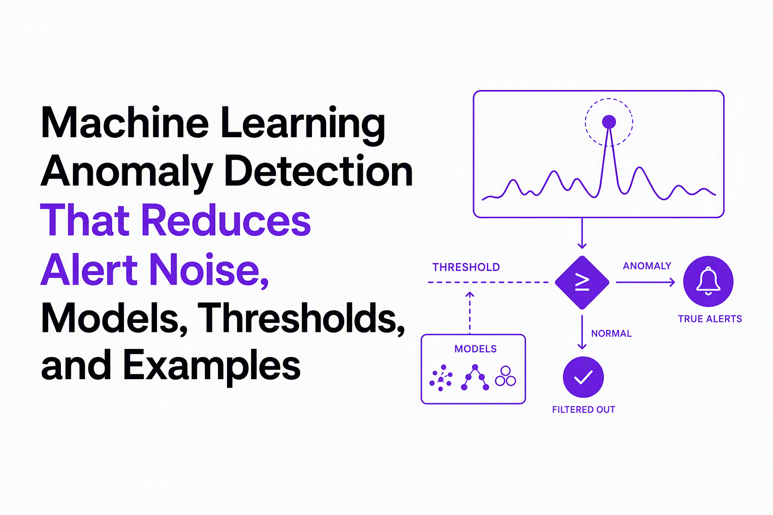
How to Evaluate, Set Thresholds, and Cut False Positives
Thresholding is the main lever for reducing false positives in machine learning anomaly detection because most models output a score, not a decision.
Use evaluation that matches the base rate and review workflow
- PR-AUC over ROC-AUC when anomalies are rare, because ROC can look good while precision is terrible.
- Precision at k for human review queues (for example, k = 20 per day per service).
- Event-level vs issue-level metrics: if you group duplicates, measure precision on grouped issues, not raw events.
Three thresholding patterns that survive production reality
- Cost-based thresholding: set a threshold where expected cost of a miss equals expected cost of a false alarm. You can do this even with rough estimates.
- Two-stage gates: a low threshold for logging and enrichment, a higher threshold for paging. This preserves recall without waking people up unnecessarily.
- Per-segment thresholds: different thresholds per endpoint, tenant tier, region, or fingerprint, because base rates differ.
Calibrate contamination assumptions instead of copying defaults
Many unsupervised methods require an implicit or explicit assumption about anomaly rate (often called contamination). We initially assumed a fixed global contamination worked, but audits showed some endpoints had near-zero true anomalies while others were naturally spiky, so per-segment calibration reduced noisy outliers without suppressing real incidents.
Make false positives measurable and reviewable
Operationally, treat every alert as a labeled data point: true incident, expected behavior, duplicate, or low-confidence. Track weekly precision and the top sources of noise, then feed changes into either features, grouping, or thresholds. A practical guide for quantifying this is false positives measurement tied to your workflow.
| Goal | Recommended metric | Threshold strategy | Common mistake |
|---|---|---|---|
| Human review queue | Precision@k | Rank anomalies, review top k daily | Paging on every score crossing |
| Paging/on-call | Precision, time-to-detect | Two-stage gates + per-segment thresholds | Single global threshold across services |
| Issue-level tracking | Grouped-issue precision | Fingerprint then threshold on group deviation | Measuring on raw event volume |
| Model comparison | PR-AUC | Choose model with stable precision under drift | Using ROC-AUC on rare anomalies |
FAQ
If your anomaly signals are technically sound but still create noisy tickets, Flash Log can help operationalize them by automatically capturing production bugs even when users do not report them, classifying events with a confidence gate, and grouping recurring failures into one issue so engineers see fewer interruptions and more actionable work.

Notification Spam Explained and How to Stop It on Any Device
Notification spam explained in plain English, with steps to find the source and stop it on iPhone, Android, browsers, email, and SMS.

Production Debugging Without a Local Repro - How to Rebuild the Missing Context
Learn a minimal reproducible context framework for production debugging when you can’t reproduce locally, and narrow hypotheses fast.
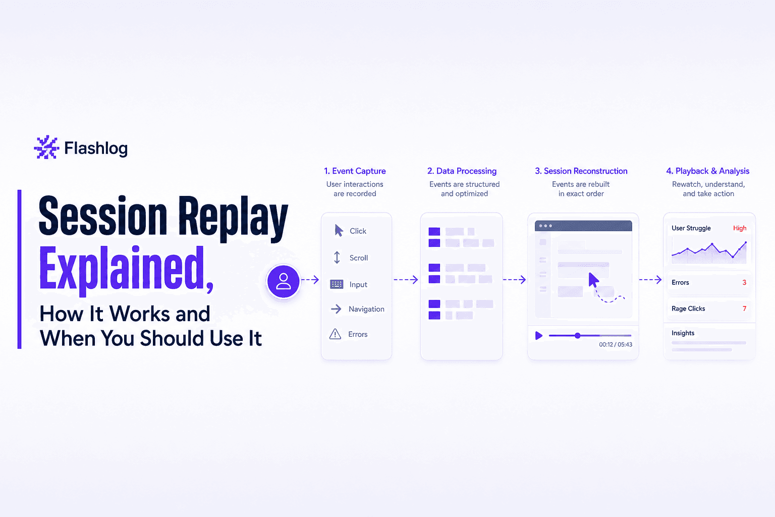
Session Replay Explained, How It Works and When You Should Use It
Learn what session replay is, how it works, top use cases, and the privacy basics you must get right before rolling it out.