
Outlier Identification That Works, The 1.5 IQR Rule, Method Selection, and Excel Steps
Outlier identification works best when you match the detection method to the outlier type, then apply a repeatable workflow: define the outlier you care about, compute flags (for example 1.5×IQR), and decide what to do with flagged points instead of auto-deleting them.
- Use 1.5×IQR for fast, distribution-agnostic outlier identification on small to medium samples, especially when you want an explainable rule.
- Pick Z-score or Grubbs/ESD only when the normality and independence assumptions are defensible, otherwise prefer MAD or IQR.
- Flagging is not the finish line: validate data quality, check sensitivity, then keep, transform, cap, or exclude with documentation.
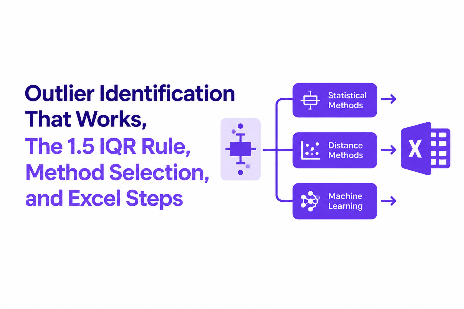
The three main types of outliers and why the type changes the detection method
Outlier type determines the right outlier identification method because “unusual compared to what” changes from a single distribution to a context window or a group pattern.
1) Global outliers (point anomalies)
Global outliers are individual points that are extreme relative to the overall dataset distribution. Analytics examples include a single order value far above typical baskets, or one response time that is far higher than the rest of the day’s traffic. Observability examples include a single API request with a 30-second latency while most requests sit below 500 ms.
Best-fit methods: IQR, MAD, Z-score (if roughly normal), Grubbs (if you truly expect one outlier and normality holds).
2) Contextual outliers (conditional anomalies)
Contextual outliers are only outliers after you condition on context such as time, cohort, endpoint, region, device, or feature flag. A 2-second response time might be normal for a cold start job but an outlier for a warmed cache read. In product analytics, a conversion rate drop can be “normal” at 3 a.m. for a small geo, but an outlier for peak hours.
Best-fit methods: run outlier identification per segment (per endpoint, per region) or on residuals after a baseline model. In practice, simple segmentation beats fancy math when the context boundary is obvious.
3) Collective outliers (group anomalies)
Collective outliers are patterns across multiple points that look normal individually but abnormal as a group, like a run of elevated error rates, a burst of retries, or 50 near-identical failures that each fall just below your threshold. This is where single-point rules often miss real incidents.
Best-fit methods: windowed detection, burst rules, and grouping by fingerprint (for errors) rather than only “is this single value extreme?”
In our experience working with production event streams, most “mysterious” misses come from treating contextual or collective behavior as if it were global, then wondering why an IQR or Z-score rule feels inconsistent across endpoints.
1.5 times IQR rule for outlier identification, full worked example from raw data to final flags
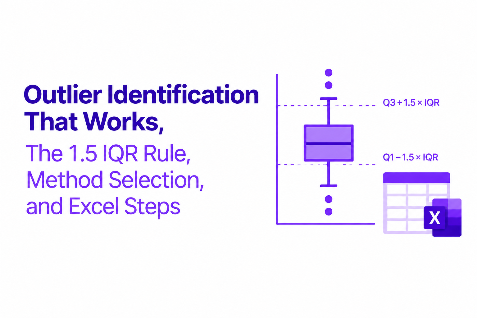
The 1.5×IQR rule is a practical outlier identification default because it does not assume normality and produces explainable upper and lower fences.
Dataset
Use this concrete dataset (20 values) so you can reproduce every step in a calculator or Excel:
8, 9, 10, 10, 11, 12, 12, 13, 13, 14, 14, 15, 15, 16, 17, 18, 19, 20, 22, 45
Step 1: Sort the data
The data above is already sorted ascending. Sorting is non-negotiable for quartile-based methods.
Step 2: Compute Q1 and Q3 using the “median of halves” approach
With n = 20 (even), split into two halves of 10 values each.
- Lower half (positions 1 to 10): 8, 9, 10, 10, 11, 12, 12, 13, 13, 14
- Upper half (positions 11 to 20): 14, 15, 15, 16, 17, 18, 19, 20, 22, 45
Q1 is the median of the lower half (average of its 5th and 6th values):
- 5th = 11
- 6th = 12
Q1 = (11 + 12) / 2 = 11.5
Q3 is the median of the upper half (average of its 5th and 6th values in that half):
- 5th = 17
- 6th = 18
Q3 = (17 + 18) / 2 = 17.5
Note: Excel’s QUARTILE.INC / QUARTILE.EXC can yield slightly different quartiles depending on interpolation rules. The fences will be close, but if you need exact agreement across tools, standardize the quartile definition in your team.
Step 3: Compute the IQR
IQR = Q3 - Q1 = 17.5 - 11.5 = 6.0
Step 4: Compute the lower and upper fences
Using the classic Tukey rule:
- Lower fence = Q1 - 1.5 × IQR = 11.5 - 1.5 × 6 = 11.5 - 9 = 2.5
- Upper fence = Q3 + 1.5 × IQR = 17.5 + 9 = 26.5
Step 5: Flag outliers and document the decision
Any value below 2.5 or above 26.5 is an outlier under this rule. In the dataset, only 45 exceeds 26.5, so it is flagged as an upper outlier; there are no lower outliers.
This is the core deliverable of outlier identification for many workflows: a reproducible rule that returns a boolean flag plus the fences you can store alongside the result.
What surprised our team the first time we operationalized IQR fences in dashboards was how often the “obvious” outliers disappeared once we segmented by endpoint or cohort, which is a reminder that many real-world problems are contextual, not global.
Choosing the right outlier identification method, IQR vs Z-score vs MAD vs Grubbs vs generalized ESD
Method choice for outlier identification comes down to four criteria you can check quickly: distribution shape, sample size, whether you expect multiple outliers, and whether you can tolerate masking and swamping.
A decision checklist (use this before picking a formula)
- Distribution: Is the data roughly symmetric and normal-like, or skewed/heavy-tailed?
- n: Are you working with n < 30, n in the hundreds, or streaming windows?
- Multiple outliers: Do you expect more than one extreme point?
- Failure mode risk: Are you worried about masking (outliers hiding each other) or swamping (non-outliers flagged)?
- Explainability: Do you need a simple fence/threshold you can communicate to non-statisticians?
Pragmatic guidance by method
- IQR (Tukey fences): Great default for skewed data and quick explainability. Can miss collective anomalies and can be too permissive if the IQR inflates due to broad variability.
- Z-score: Useful when the data is approximately normal and you need a standardized distance from the mean. Breaks down with skew and heavy tails because mean and standard deviation are not robust.
- MAD (median absolute deviation): Robust alternative to Z-score: replace mean with median and std dev with MAD-derived scale. Strong choice when you suspect heavy tails or genuine extreme values that should not distort the scale.
- Grubbs test: Hypothesis test for a single outlier under normality assumptions. Not designed for multiple outliers without iterative approaches, and it can be sensitive to violations of normality.
- Generalized ESD (Extreme Studentized Deviate): Extension for multiple outliers. Still leans on normality and independence; in operational data, independence is often the first assumption to fail.
Masking and swamping, the two ways outliers break your detector
Masking happens when multiple outliers pull the mean and standard deviation (or other statistics) so far that each outlier looks less extreme, especially in Z-score-based approaches. Swamping happens when the method’s scale estimate is too small or the distribution is skewed, causing many normal points to be labeled as outliers.
When we tested Z-scores on latency data with long tails, the practical outcome was predictable: we either set a high threshold that missed real regressions or a low threshold that flooded the review queue. Switching to MAD or segment-specific IQR fences was usually the cleaner trade.
| Method | Assumptions (practical) | Handles multiple outliers? | Best for | Main failure mode |
|---|---|---|---|---|
| IQR (1.5×) | No normality required; needs stable quartiles | Yes (rule-based) | Skewed data, simple fences, quick reviews | Context mixing; misses collective patterns |
| Z-score | Rough normality; mean and std dev meaningful | Yes (but prone to masking) | Quality control, stable symmetric distributions | Heavy tails cause high false positives |
| MAD (robust Z) | Few; works well under skew/heavy tails | Yes | Operational metrics, robust thresholding | Less familiar; needs careful scaling constant |
| Grubbs | Normality; typically one outlier | No (by design) | Small samples when you truly expect one bad point | Misleading under non-normality |
| Generalized ESD | Normality; independent observations | Yes | Multiple outliers in controlled measurements | Assumptions often fail in time series |
How to calculate and label outliers in Excel using QUARTILE, MEDIAN, STDEV, and conditional logic
Excel outlier identification is easiest to maintain when you store the fences in dedicated cells and label each row with an explicit status like LOWER, NORMAL, or UPPER.
Worksheet pattern (copy-friendly)
Assume your values are in A2:A21 (20 rows). Put these in cells:
- Q1 (C2):
=QUARTILE.INC($A$2:$A$21,1) - Q3 (C3):
=QUARTILE.INC($A$2:$A$21,3) - IQR (C4):
=C3-C2 - Lower fence (C5):
=C2-1.5*C4 - Upper fence (C6):
=C3+1.5*C4
Row label formula
In B2, then fill down:
=IF(A2<$C$5,"LOWER_OUTLIER",IF(A2>$C$6,"UPPER_OUTLIER","NORMAL"))
If you need Z-score labels (and the distribution supports it)
- Mean (D2):
=AVERAGE($A$2:$A$21) - Std dev (D3):
=STDEV.S($A$2:$A$21) - Z (E2):
=(A2-$D$2)/$D$3 - Flag at |Z| > 3 (F2):
=IF(ABS(E2)>3,"OUTLIER","NORMAL")
For robust MAD in Excel, you can compute the median and then the median of absolute deviations using helper columns (Excel does not provide a one-cell MAD function). If you are building something long-lived, I usually keep IQR fences for the spreadsheet workflow and move MAD to a scripted pipeline where the implementation is less fragile.
When an outlier is signal not noise, a decision flow for validate, keep, transform, or exclude
A flagged point becomes useful only after a decision flow that separates data errors, expected extremes, and true rare events worth acting on.
A 4-step decision flow you can run in under 15 minutes
- Validate the record (data quality check): confirm units, timestamp, joins, null handling, and deduplication. If the point came from instrumentation, verify the client and server clocks and whether retries were counted as unique events.
- Check context: segment by the most obvious drivers (endpoint, region, device, plan, feature flag). If the outlier disappears inside a segment, you likely had a contextual outlier, not a global one.
- Sensitivity test: rerun the summary metric or model with and without the flagged points. If the business conclusion flips, treat this as a modeling risk and justify the handling explicitly.
- Choose handling and document it: keep as-is (rare but real), transform (log, winsorize/cap), isolate (separate distribution), or exclude (only with a clear rationale and traceability).
What to do in common scenarios
- Data entry or pipeline bug: fix upstream, backfill, exclude from analysis, and log a clear exception note with the rule used.
- Expected extremes (business rules): keep, but consider separate reporting. Example: declined payments, validation failures, and permission denials are often expected responses, not defects.
- True incident signal: keep and escalate, but group duplicates so you do not create a storm of identical tickets. Collective outliers are operationally expensive when you treat each event as unique.
- Long-tailed distributions: prefer MAD or percentile-based thresholds, or use IQR per segment. Z-score flags often become a proxy for “tail exists” rather than “something broke.”
Operationalizing the flow for observability and bugs
In practice, the hardest part is not computing fences, it is stopping flagged points from becoming noisy work. That is why teams often pair statistical outlier identification with a decision layer: ignore known harmless patterns, group repeated failures into one thread, and hold back low-confidence signals until more context arrives.
For related workflows on detection in production systems, see outlier detection, anomaly detection, and alert triage. If false alarms are your main pain, false positives usually come from context mixing, duplicate storms, or thresholds chosen without a decision plan.
FAQ
If you want to apply outlier identification to real production behavior without turning every odd event into noisy work, Flash Log can help operationalize the last mile by automatically capturing bugs even when users do not report them and using AI classification to separate real defects from expected failures, duplicates, and low-confidence signals so engineering only sees actionable issues.

Web Session Replay Explained With a Step-by-Step Setup and One Real Debugging Example
Learn web session replay fundamentals: what it captures, how it works, and a step-by-step setup plus a real timeline walkthrough to find root cause.

Adaptive Sampling for Observability, A Practical Framework to Cut Noise Without Missing Incidents
Adaptive sampling framework for observability: pick signals, set rates with SLO risk math, validate quality, and cut telemetry noise without hiding incidents.

Bug Detection for Support Teams, A Proactive Workflow to Catch Issues Before Users Report Them
Build proactive bug detection for Support with clear signals, triage rules, evidence standards, and a weekly cadence that engineering trusts.