
Outlier Detection in Practice, A Workflow for Methods, Formulas, and Thresholds
Outlier detection is most reliable when you treat it as a workflow (from visualization to safe action) instead of a one-off threshold guess, because the right method and cutoff depend on distribution shape, dimensionality, and the cost of false alarms versus missed outliers.
- Start with a repeatable workflow: visualize, characterize, choose univariate vs multivariate, then decide how to act safely.
- Pick formulas based on assumptions: IQR and MAD for skew and heavy tails, z-score for near-normal, Mahalanobis or robust models for multivariate.
- Set thresholds by cost (false positives vs misses) and validate on backtests before routing anything to engineers.
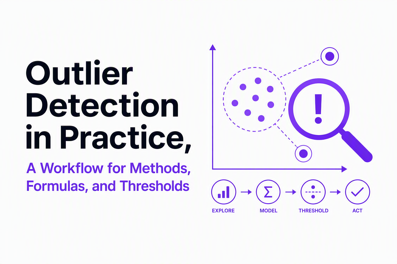
A repeatable outlier detection workflow from plot to action
A practical outlier detection workflow reduces guesswork by forcing each choice (method, threshold, and action) to match the data shape and the business cost of getting it wrong.
Step 1: Visualize in a way that reveals failure modes
Use plots that show both tails and density, not just central tendency. For univariate signals, a histogram plus a log-scaled y-axis often surfaces rare event clusters; a box plot quickly shows tail heaviness but can hide multimodality. For time series, plot residuals after subtracting trend/seasonality (even a simple rolling median) before labeling points as outliers.
Step 2: Characterize the distribution and the “unit of analysis”
Write down three facts before selecting a detector: (1) is the signal roughly symmetric, skewed, or multi-peak, (2) are outliers isolated points or bursty segments, and (3) what is one observation, for example per request, per user-session, per minute bucket. In our experience, half of “bad thresholds” were really mismatched units, like scoring per request but alerting per minute without aggregating.
Step 3: Decide univariate vs multivariate (and avoid mixing them)
Use univariate methods when one feature explains the risk, such as latency, amount, or error rate. Use multivariate methods when “weirdness” is a combination, such as (latency high AND payload small AND route unusual). If you only have a few features and you care about correlation structure, multivariate can cut false positives dramatically, but only if you standardize and handle missing values consistently.
Step 4: Choose the action path before you choose the threshold
Every outlier label should map to an action: log-only, create an investigation task, page on-call, or block a transaction. Decide whether you need “novelty detection” (train on clean baseline, flag anything different later) or “outlier detection” (assume training data contains anomalies). This choice directly impacts model selection and evaluation.
Outlier detection formulas cheat sheet, what to use when
Outlier detection formulas are only as good as their assumptions, so the fastest way to choose is to match each method to distribution shape, sample size, and whether you need robustness to heavy tails.
Cheat sheet: formulas, assumptions, and pitfalls
- IQR rule (boxplot rule): Flag if x < Q1 - 1.5·IQR or x > Q3 + 1.5·IQR, where IQR = Q3 - Q1. Use for skewed data and when you want a simple, nonparametric rule. Pitfall: for very heavy-tailed distributions, it can over-flag.
- Z-score: z = (x - μ)/σ, flag if |z| > k. Use when data is approximately normal and stable. Pitfall: μ and σ are sensitive to outliers; a few extreme points can “hide” each other by inflating σ.
- Modified z-score (MAD): M = 0.6745·(x - median)/MAD, where MAD = median(|x - median|). Use for heavy tails and skew, robust to contamination. Pitfall: if MAD is near zero (many identical values), you need smoothing or an alternate scale.
- Mahalanobis distance: D² = (x - μ)ᵀ Σ⁻¹ (x - μ). Use for multivariate data with roughly elliptical contours. Pitfall: Σ is unstable in high dimensions or with collinearity; consider shrinkage or robust covariance.
- Grubbs’ test / Generalized ESD: hypothesis tests for one or multiple outliers under normality assumptions. Use in QA-style batch checks with small n and strong distribution assumptions. Pitfall: not ideal for streaming, and results depend heavily on normality.
Quick selection checklist (what we actually do)
- If the histogram is skewed or has long tails: start with MAD or IQR.
- If you have clear normal behavior and stable variance: z-score is fine, but compute μ and σ on a clean window.
- If correlations matter (for example, “rare combo” patterns): Mahalanobis or a robust multivariate model.
- If you must justify statistically in an audit context: Grubbs/ESD, but validate normality and sample size.
Thresholds without guessing, unify alpha, contamination, and z cutoffs using cost
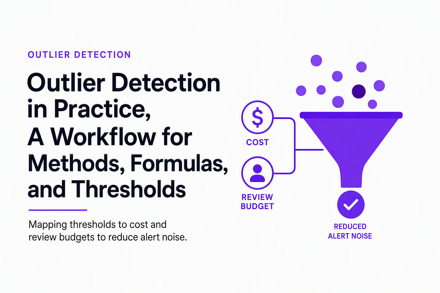
Threshold setting for outlier detection becomes tractable when you translate it into a cost decision: how expensive is a false positive compared to a missed outlier, and what volume of review work can you afford.
A cost-based framework you can apply to any detector
Most threshold knobs are the same idea in different packaging:
- z cutoff (k): how extreme a point must be
- alpha (stat tests): acceptable false alarm probability under assumptions
- contamination (many ML detectors): expected fraction of outliers
Convert business constraints into an operational target, then map to your knob:
- Set a review budget: for example, “we can manually review 20 events per day” or “we can tolerate 1 Slack alert per hour.”
- Set a miss tolerance: what happens if you miss one true outlier, such as lost revenue, broken checkout, or security risk. If misses are costly, bias toward recall and add a second-stage filter to reduce noise.
- Backtest thresholds on a holdout period with known incidents or proxy labels (customer complaints, rollbacks, confirmed bugs).
- Choose the threshold that meets the review budget while capturing the incidents you care about, not the one that “looks statistically nice.”
A concrete sigma-rule mapping (and why it fails)
If a metric is close to normal, |z| > 3 corresponds to about 0.27% of points in both tails under ideal assumptions. That sounds like a clean default, but it fails when (1) the distribution is heavy-tailed, (2) variance changes by time-of-day, or (3) you are scanning hundreds of metrics, where even tiny false positive rates add up. Our team initially assumed “3-sigma is conservative,” but in production telemetry it often created steady background noise because the tails were not normal.
Practical guardrails to keep thresholds stable
- Compute thresholds on a rolling baseline window and freeze them for an evaluation window to avoid chasing noise.
- Use per-segment thresholds (route, tenant, device class) only when each segment has enough volume; otherwise you overfit and explode false alarms.
- Separate “detection threshold” from “notification threshold”: detect more, alert less, and aggregate before paging.
Multivariate and high-dimensional methods that actually work in practice
Multivariate outlier detection works best in practice when you standardize features, avoid leakage, and pick algorithms that match your operational mode (novelty vs contamination) and data geometry.
What to use and when (decision criteria)
- Isolation Forest: strong default for tabular, scales well, works without distance metrics. Good when you want a ranked anomaly score and can set contamination to meet a review budget.
- Local Outlier Factor (LOF): good when “outliers are local,” meaning they deviate from a neighborhood, not globally. Works best with well-scaled, meaningful distances.
- One-Class SVM: can work on smaller datasets with careful kernel tuning; sensitive to scaling and parameter choices. Use when you truly have mostly-clean baseline data (novelty detection).
- EllipticEnvelope (robust covariance): interpretable when data is roughly elliptical. Breaks down with many correlated features unless regularized.
Operational pitfalls that cause false alarms
- Scaling mismatch: always standardize numeric features; consider log transforms for long-tail variables (amounts, latencies).
- Data leakage: do not include features that encode the label indirectly, like “error_message_hash” if you want to detect unknown failures.
- Mode mismatch: LOF’s novelty mode differs by implementation; for streaming, prefer algorithms and APIs designed for novelty detection if you train on clean history.
How this ties to engineering noise in production systems
High-dimensional detectors are great at surfacing rare combinations, but raw scores should not directly create tickets. A safer pattern is: score events, aggregate by fingerprint (same root cause), then route only high-confidence clusters. This is the same decision-layer idea used in noise control systems: separate expected failures and duplicates from the issues engineers should actually work.
Python patterns you can copy, scores, labels, and evaluation
Copy-paste Python patterns make outlier detection repeatable because they enforce a consistent flow: fit baseline, compute scores, pick a threshold by budget, then evaluate on incidents or proxies.
Pattern 1: IQR and MAD for robust univariate detection
import numpy as np

x = np.asarray(values, dtype=float)

# IQR rule
q1, q3 = np.percentile(x, [25, 75])
iqr = q3 - q1
lower, upper = q1 - 1.5 * iqr, q3 + 1.5 * iqr
iqr_flags = (x < lower) | (x > upper)

# Modified z-score (MAD)
med = np.median(x)
mad = np.median(np.abs(x - med))
if mad == 0:
    mad = np.mean(np.abs(x - med)) + 1e-9  # fallback scale
mod_z = 0.6745 * (x - med) / mad
mad_flags = np.abs(mod_z) > 3.5
Pattern 2: Isolation Forest with a review-budget threshold
import numpy as np
from sklearn.ensemble import IsolationForest
from sklearn.preprocessing import StandardScaler
from sklearn.pipeline import Pipeline

X = features  # shape (n_samples, n_features)

pipe = Pipeline([
    ("scaler", StandardScaler()),
    ("iso", IsolationForest(
        n_estimators=300,
        contamination=0.01,  # start with a guess, then tune by budget
        random_state=42
    ))
])

pipe.fit(X)
# score_samples: higher is more normal; decision_function similar
scores = pipe.named_steps["iso"].score_samples(pipe.named_steps["scaler"].transform(X))

# Turn scores into top-K review list (budget-driven)
K = 50  # e.g., review 50 worst per day/batch
worst_idx = np.argsort(scores)[:K]
review_candidates = X[worst_idx]
Pattern 3: LOF for local deviations (use carefully)
import numpy as np
from sklearn.neighbors import LocalOutlierFactor
from sklearn.preprocessing import StandardScaler

X = features
Xz = StandardScaler().fit_transform(X)

lof = LocalOutlierFactor(n_neighbors=35, contamination=0.01)
labels = lof.fit_predict(Xz)  # -1 outlier, 1 inlier
lof_scores = -lof.negative_outlier_factor_  # higher means more outlier-ish
Evaluation that works when you lack perfect labels
- Incident overlap: compare flagged windows with known outages, bug reports, or rollback timestamps.
- Stability checks: thresholds should not swing wildly week to week unless the system changed.
- Precision proxy: sample 30 to 100 flagged events and categorize them as actionable vs expected. Use that to tune thresholds and ignore rules.
To reduce alert noise specifically, we usually measure “alerts per day per service” and “unique root causes per alert.” If the first is high and the second is low, you need aggregation and deduping more than a new model.
For deeper workflows on detection and noise, see anomaly detection, detection of anomalies, and how to cut false positives with better routing and review design.
| Goal | Recommended method | Threshold knob | Best practice to reduce noise |
|---|---|---|---|
| Robust univariate tails | MAD (modified z) or IQR | |M| > 3.5 or 1.5·IQR | Segment only when you have enough volume per segment |
| Correlated multivariate patterns | Isolation Forest | contamination or top-K | Rank then group by fingerprint before creating tickets |
| Local neighborhood deviations | LOF | contamination | Standardize, tune neighbors, and validate on a holdout period |
| Audit-style statistical testing | Grubbs / ESD | alpha | Verify normality assumptions and use offline batches |
FAQ
If you want to operationalize outlier detection in production without turning every weird event into engineering noise, Flash Log adds a decision layer that auto-captures bugs even when users never report them, classifies signals with AI plus rules, and groups duplicates into one clean issue so only actionable outliers reach Jira, Linear, Slack, or weekly reviews.

Bug Tracking for Support Teams, A Practical Workflow From Intake to Verified Fix
Bug tracking playbook for support teams: owners, templates, SLAs, and KPIs to turn noisy tickets into verified fixes and reduce defect leakage.

Software Bug Tracking System Buyer Guide, How To Choose The Right One In 2026
A practical 2026 buyer guide to pick a software bug tracking system using criteria, a shortlist by use case, and a rollout checklist.
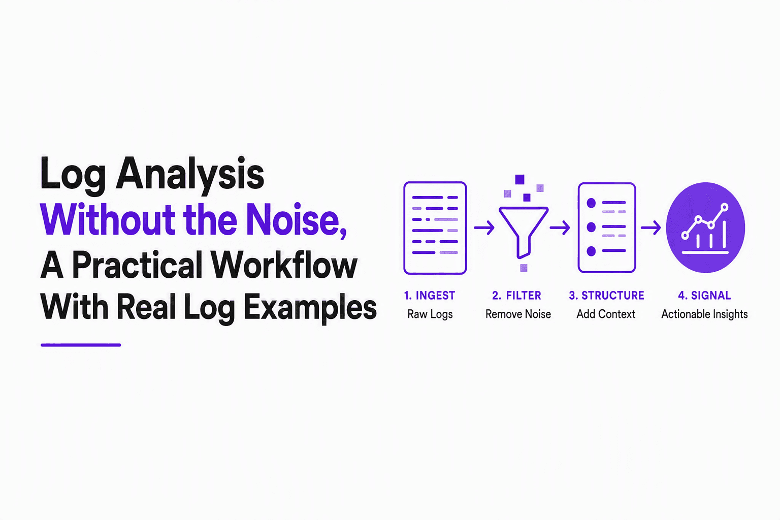
Log Analysis Without the Noise, A Practical Workflow With Real Log Examples
Learn log analysis without alert fatigue: a repeatable workflow, real log examples, Linux commands, and AI noise reduction guardrails.